1. CNN에 대해서 조금 정리하고 넘어가자.
- input image 14x14x3 이 있고, filter가 5x5x3 이고 개수가 20이라고 하자.
- 여기서 하나의 필터는 input image에서 '어떠한' 특성을 잡아낸다(세로선이든 대각선이든. 물론 층이 깊어질 수록 그런 단순한 수준보다는 더 복잡한 패턴을 인식하겠지 어찌됐든 뭔가 feature를 잡아낸다).
- 필터가 20개이므로 20개의 특성을 잡아내는 것.
- 이 연산의 결과로 10x10x20 이 산출된다.
- 이 산출값의 channel(20개) 각각은 서로 다른 filter가 씌워진 결과로서, channel 별로 다른 feature 를 capture(?) 한 것이다. 말로 표현하기 어렵네.
- Neural Style Transfer에서 채널별로 다른 feature에 반응하므로 그 channel 간의 상관관계를 계산함으로써 style을 수치화하였다.
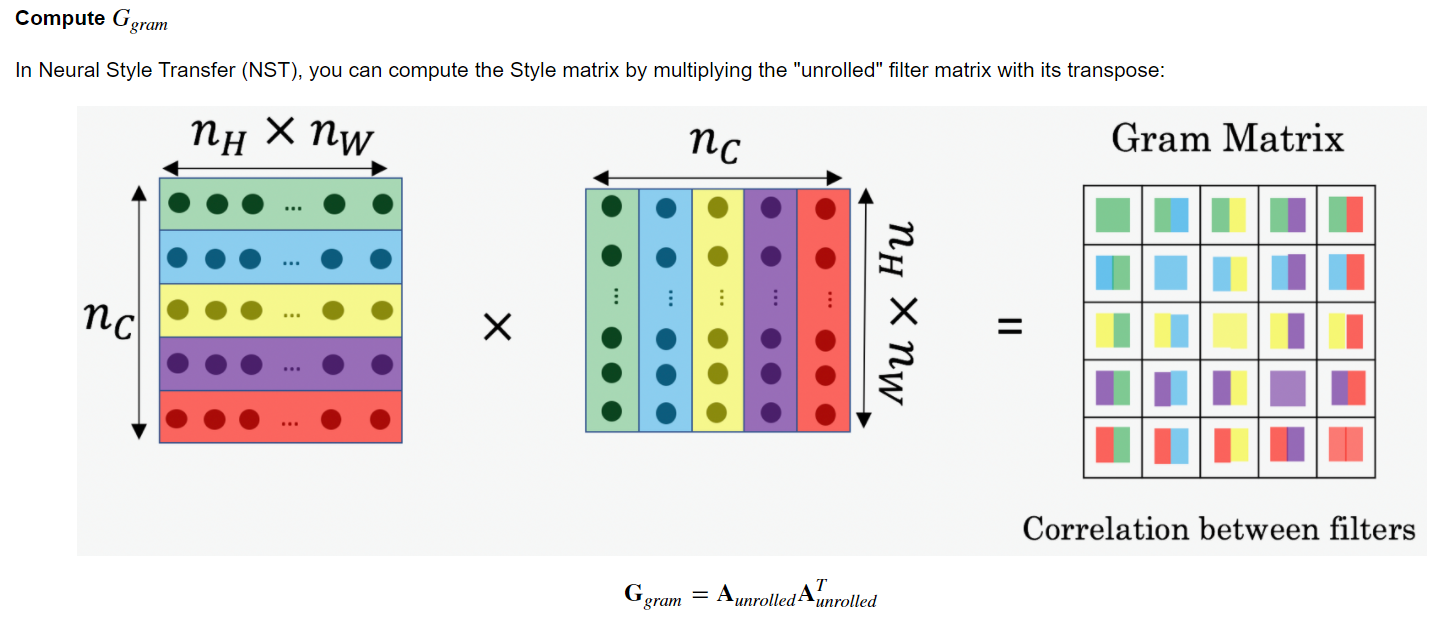
2. 사실 Unrolling은 content cost 구할 때는 필요없긴한데 style cost 구할 때 필요하므로 그냥 같이 적용시킨다. Unrolling 하는 구체적인 방법은 다음과 같다.
Exercise: Compute the "content cost" using TensorFlow.
Instructions: The 3 steps to implement this function are:
- Retrieve dimensions from a_G:
- To retrieve dimensions from a tensor X, use: X.get_shape().as_list()
- Unroll a_C and a_G as explained in the picture above
- You'll likey want to use these functions: tf.transpose and tf.reshape.
- Compute the content cost:
- You'll likely want to use these functions: tf.reduce_sum, tf.square and tf.subtract.
Additional Hints for "Unrolling"
- To unroll the tensor, we want the shape to change from (m,nH,nW,nC)(m,nH,nW,nC) to (m,nH×nW,nC)
- tf.reshape(tensor, shape) takes a list of integers that represent the desired output shape.
- For the shape parameter, a -1 tells the function to choose the correct dimension size so that the output tensor still contains all the values of the original tensor.
- So tf.reshape(a_C, shape=[m, n_H * n_W, n_C]) gives the same result as tf.reshape(a_C, shape=[m, -1, n_C]).
- If you prefer to re-order the dimensions, you can use tf.transpose(tensor, perm), where perm is a list of integers containing the original index of the dimensions.
- For example, tf.transpose(a_C, perm=[0,3,1,2]) changes the dimensions from (m,nH,nW,nC)(m,nH,nW,nC) to (m,nC,nH,nW)(m,nC,nH,nW).
- There is more than one way to unroll the tensors.
- Notice that it's not necessary to use tf.transpose to 'unroll' the tensors in this case but this is a useful function to practice and understand for other situations that you'll encounter.
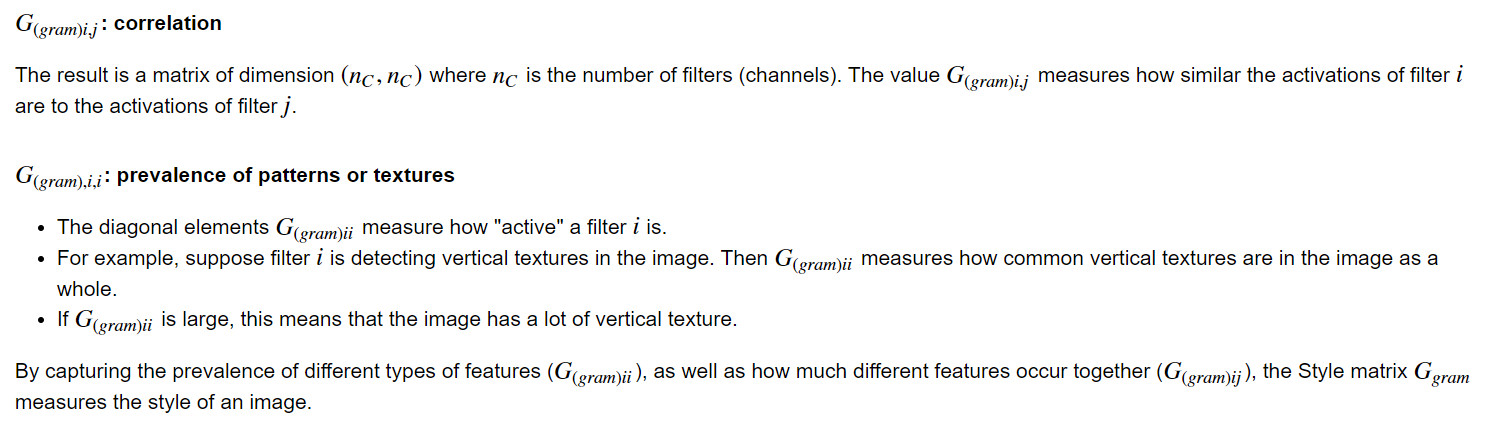
3. G(i,i) 의 의미:
Gram Matrix 가 channel 간 상관관계를 의미한다는 것을 배웠다. 그렇다면 G(i,i) 즉, 같은 channel 끼리 곱해져 더해진 것은 무엇을 의미할까? 바로 prevalence of patterns or textures 이다. 즉, 해당 channel이 특정 feature 를 detect하는 filter 의 결과값일 때, G(i,i) 값은 feature의 activity 정도이다. 아래 예시를 참조.
4. Unrolling
def compute_layer_style_cost(a_S, a_G):
    """
    Arguments:
    a_S -- tensor of dimension (1, n_H, n_W, n_C), hidden layer activations representing style of the image S
    a_G -- tensor of dimension (1, n_H, n_W, n_C), hidden layer activations representing style of the image G

    Returns:
    J_style_layer -- tensor representing a scalar value, style cost defined above by equation (2)
    """

    ### START CODE HERE ###
    # Retrieve dimensions from a_G (≈1 line)
    m, n_H, n_W, n_C = a_G.get_shape().as_list()

    # Reshape the images to have them of shape (n_C, n_H*n_W) (≈2 lines)
    a_S = tf.reshape(tf.transpose(a_S, perm = [0,3,1,2]), shape = [n_C, n_H*n_W])
    a_G = tf.reshape(tf.transpose(a_G, perm = [0,3,1,2]), shape = [n_C, n_H*n_W])

    # Computing gram_matrices for both images S and G (≈2 lines)
    GS = gram_matrix(a_S)
    GG = gram_matrix(a_G)

    # Computing the loss (≈1 line)
    J_style_layer = (1/(4*np.square(n_C)*np.square(n_H)*np.square(n_W))) * tf.reduce_sum(tf.square(tf.subtract(GS,GG)))

    ### END CODE HERE ###

    return J_style_layer
Unrolling 할 때, 차원을 [n_C, n_H*n_W] 로 바꾸어야 한다. 하지만 기존 a_S와 a_G의 배열은 [1, n_H, n_W, n_C] 이므로 reshape로 바로 바꿀 수가 없다. 그렇게 되면 원하는 모양은 나오지만 그 구성은 원하지 않는 결과물이 나온다.
따라서 transpose로 먼저 구성을 유지한 채로 reshape 하고자 하는 순서로 차원을 바꿔주고 reshape 한다. 무슨 말인지는 코드를 보면 알 수 있다.
5. 가중치
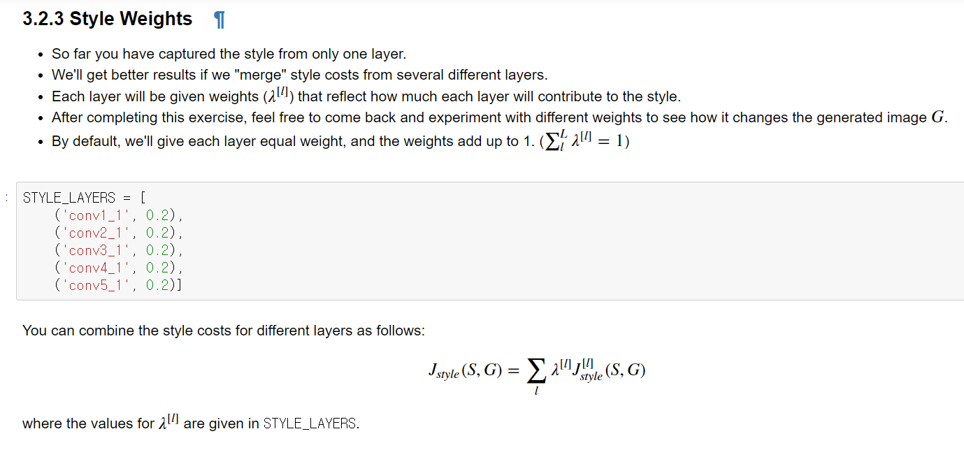
sum of weights = 1 이다. 어차피 나중에 style cost와 content cost 의 비율을 알파와 베타로 조절하기는 하지만, 일단 1로 하여 시작은 동등하게 하기 위함인듯.
5. a_G 정의
def compute_style_cost(model, STYLE_LAYERS):
    """
    Computes the overall style cost from several chosen layers

    Arguments:
    model -- our tensorflow model
    STYLE_LAYERS -- A python list containing:
                        - the names of the layers we would like to extract style from
                        - a coefficient for each of them

    Returns:
    J_style -- tensor representing a scalar value, style cost defined above by equation (2)
    """

    # initialize the overall style cost
    J_style = 0

    for layer_name, coeff in STYLE_LAYERS:

        # Select the output tensor of the currently selected layer
        out = model[layer_name]

        # Set a_S to be the hidden layer activation from the layer we have selected, by running the session on out
        a_S = sess.run(out)

        # Set a_G to be the hidden layer activation from same layer. Here, a_G references model[layer_name]
        # and isn't evaluated yet. Later in the code, we'll assign the image G as the model input, so that
        # when we run the session, this will be the activations drawn from the appropriate layer, with G as input.
        a_G = out

        # Compute style_cost for the current layer
        J_style_layer = compute_layer_style_cost(a_S, a_G)

        # Add coeff * J_style_layer of this layer to overall style cost
        J_style += coeff * J_style_layer

    return J_style
저어기 a_G 를 out 으로 저장한 부분을 보라. 아직 우리는 모델에 image 를 input 하지 않았으므로 out 은 형태만 존재할 뿐 값이 없다. 일단 그 특정 layer 의 activation 을 out 이라고 해놓고, 아직 Generated Image 가 input 되지 않았지만, a_G로서 저장해놓고 style_cost 를 계산하기 위해 사용한다.
Note: In the inner-loop of the for-loop above, a_G is a tensor and hasn't been evaluated yet. It will be evaluated and updated at each iteration when we run the TensorFlow graph in model_nn() below.
6. Neural Style Transfer 대략적 흐름
Here's what the program will have to do:
- Create an Interactive Session
- Load the content image
- Load the style image
- Randomly initialize the image to be generated
- Load the VGG19 model
- Build the TensorFlow graph:
- Run the content image through the VGG19 model and compute the content cost
- Run the style image through the VGG19 model and compute the style cost
- Compute the total cost
- Define the optimizer and the learning rate
- Initialize the TensorFlow graph and run it for a large number of iterations, updating the generated image at every step.
7. TensorFlow 기본
[러닝 텐서플로]Chap03 - 텐서플로의 기본 이해하기
Chap03 - 텐서플로의 기본 이해하기 텐서플로의 핵심 구축 및 동작원리를 이해하고, 그래프를 만들고 관리하는 방법과 상수, 플레이스홀더, 변수 등 텐서플로의 '구성 요소'에 대해 알아보자. 3.1
excelsior-cjh.tistory.com
8. Face Verification & Recognition
Face recognition problems commonly fall into two categories:
- Face Verification - "is this the claimed person?". For example, at some airports, you can pass through customs by letting a system scan your passport and then verifying that you (the person carrying the passport) are the correct person. A mobile phone that unlocks using your face is also using face verification. This is a 1:1 matching problem.
- Face Recognition - "who is this person?". For example, the video lecture showed a face recognition video of Baidu employees entering the office without needing to otherwise identify themselves. This is a 1:K matching problem.
'DeepLearning Specialization(Andrew Ng) > Convolutional Neural Networks' 카테고리의 다른 글
| [Week 4] 2. Neural Style Transfer (0) | 2020.11.16 |
|---|---|
| [Week 4] 1. Face recognition (0) | 2020.11.14 |
| [Week 3] Quiz & Programming Assignments (0) | 2020.11.13 |
| [Week 3] 1. Detection Algorithm (0) | 2020.11.12 |
| [Week 2] Programming assignments (0) | 2020.11.09 |


